Was recently looking at anomaly detection methods and found a couple of them based on this theory I have not had the opportunity to look more closely at. So here we are. EVT is a theory of the behavior of tails of distributions. Pretty handy in risk assessment or to make decisions around extreme situations that might occur.
Will try to give a summary of what I learnt and with pointers to the source of truth in case I missed something and also references to things I have not fully grasped yet but still looks cool.
Distribution of extremes
Ever wondered what is the distribution of the maximum of \(n\) samples from the distribution? It’s actually fairly easy. Let’s define \(M_n = max(X_1, ... X_n)\), we are interested in the cumulative distribution function (cdf) of \(M_n\): \(Pr(M_n \leq x)\).
\[ \begin{aligned} Pr(M_n \leq x) &= Pr(X_1 \leq x, X_2 \leq x, \ldots X_n \leq x) \\ &= Pr(X_1 \leq x)Pr(X_2 \leq x) \ldots Pr(X_n \leq x) && \text{$X$ are i.i.d}\\ &= F(x)^n && \text{where $F(x)$ is the cdf of $X_n$}.\\ \end{aligned} \]
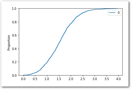
And indeed with a standard normal distribution and \(n = 10\), for the empirical CDF, we get:
# Imports
import numpy as np
import seaborn as sns
import pandas as pd

# Empirical CDF of maxima - from standard normal.
X = pd.DataFrame([np.random.normal(size=10).max() for _ in range(1000)])
sns.ecdfplot(X)
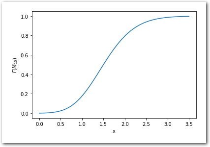
And now from the known CDF:
# More imports
import math
from scipy.special import erf

# CDF of maxima - from standard normal cdf.
x = np.linspace(0, 3.5, 100)
cdf_x = 1/2*(1 + erf(x/math.sqrt(2)))
cdf_max_of_10 = np.power(cdf_x, 10)

sns.lineplot(data=pd.DataFrame({'x': x,
                                '$F(M_{10})$': cdf_max_of_10}),
             x='x',
             y='$F(M_{10})$')
Okay, now what if we don’t know \(F(x)\).
EVT gives asymptotic results about extremes.
You are probably familiar with the central limit theorem (CLT) and its asymptotic result on \(\bar{X}_n = \sum_{i=1}^{n} {X}_i\) of \(n\) iid r.v. drawn from a distribution with finite first and second moments, respectively \(\mu\) and \(\sigma^2\). CLT says that: \[\sqrt{n}\left(\bar{X}_n - \mu\right)\ \xrightarrow{d}\ \mathcal{N}\left(0,\sigma^2\right) \text{ as } n \rightarrow \infty.\]
This is very useful and gives a convergence in distribution of the empirical mean to a Normal distribution even without us knowing the distribution of each r.v.
The first theorem of EVT – aka Fisher–Tippett–Gnedenko theorem – gives us something similar for the maximum \(M_n\) as \(n \rightarrow \infty\). This theorem is the heart of ‘Block Maxima’ method we will discuss in next section. EVT has a second ‘main’ theorem which lead to another method and this will be topic of a following post. Probably also spending some time on a couple of applications – and writing some code!
Block Maxima method
What Fisher–Tippett–Gnedenko theorem says – quoting wikipedia:
The maximum of a sample of iid random variables after proper renormalization can only converge in distribution to one of 3 possible distributions, the Gumbel distribution, the Fréchet distribution, or the Weibull distribution.
Back to our family \({X}_1,{X}_2 \ldots{X}_n\) of \(n\) iid r.v., Fisher-Tippett-Gnedenko theorem states that if there exists two sequences \(a_n \mathbb{R}_{+}^{*}\) and \(b_n \in \mathbb{R}\) such that \(Pr(\frac{max(X_1, ... X_n) - b_n}{a_n} \leq x) \xrightarrow\ G(x) \text{ as } n \rightarrow \infty\) for a non-degenerate distribution function \(G\), then \(G\) has the form:
\[G_{\mu, \sigma, \xi}(x) = exp \Bigg\{ -\left[ 1 + \xi(\frac{x - \mu}{\sigma})\right]^{-1/\xi}\Bigg\}\] with \(\mu, \xi \in \mathbb{R}\) and \(\xi \in \mathbb{R}_{+}^{*}\) and is defined on \(\{x: 1 + \xi(x-\mu)/\sigma > 0\}\). \(G\) is called GEV and is a family that contains the 3 possible distributions we mentioned earlier: Gumber, Fréchet and Weibull.
See Theorem 3.1.1 of An Introduction to Statistical Modeling of Extremes Values, Stuart Coles
Granted it’s a bit more complicated than CLT but well, it’s about maxima, and it is not without similarity: normalization, convergence in distribution to know ‘shapes’.
From a practical standpoint, the series \(a_n\) and \(b_n\) can be intimidating at first as it seems it is something we will need to pull out of our hat – or wherever you store your stock of unknown series. They are actually not a concern once we note that we don’t know the parameters \(\mu, \sigma, \xi\) – will be looking for them, and observing that under the convergence assumption, we can get them disappear in the RHS by reparameterizing \(G\).
In the end, under the convergence assumption, we are looking for \(\mu, \sigma, \xi\) such that \(G_{\mu, \sigma, \xi}\) approximates our distribution of maxima.
The Block Maxima (BM) method leverages this results in a pretty straightforward manner once we noted we can create our own maximum by defining blocks and computing the maximum therein, and we can ‘fit’ \(G_{\mu, \sigma, \xi}\) with a standard method like MLE or Bayesian inference.
Will skip the technical details on pitfalls of using MLE here and point you to the section 3.3.2 from the book of Stuart Coles for more information on this topic - Bayesian inference is discussed in the book too. Note also that this theorem doesn’t provide the condition for the convergence. It provides the family the limiting distribution belongs too IF there is convergence. More on the convergence conditions here or Proposition 2.9 here – they are known as von Mises conditions.
Before moving on: there are extensions of this to non-i.i.d sequences, non-stationary and multivariate cases too.
Next
A common observation is that BM is wasting data if we have more than just the maxima for each blocks. POT addresses that by considering the data over a certain threshold - hence the name ‘Peaks Over Threshold’.
